SignacX, Seurat and MASC: Analysis of kidney cells from AMP
Compiled 2021-03-02
Source:vignettes/signac-Seurat_AMP.Rmd
signac-Seurat_AMP.RmdSometimes, we have single cell genomics data with disease information, and we want to know which cellular phenotypes are enriched for disease. In this vignette, we applied SignacX to classify cellular phenotypes in healthy and lupus nephritis kidney cells, and then we used MASC to identify which cellular phenotypes were disease-enriched.
Note:
- MASC typically requires equal numbers of cells and samples between case and control: an unequal number might skew the clustering of cells towards one sample (i.e., a “batch effect”), which could cause spurious disease enrichment in the mixed effect model. Since Signac classifies each cell independently (without using clusters), Signac annotations can be used with MASC without a priori balancing samples or cells, unlike cluster-based annotation methods.
This vignette shows how to use SignacX with Seurat and MASC. There are three parts: Seurat, SignacX and then MASC. We use an example data set of kidney cells from AMP from this publication.
Load data
Read the CEL-seq2 data.
ReadCelseq <- function(counts.file, meta.file) {
    E = suppressWarnings(readr::read_tsv(counts.file))
    gns <- E$gene
    E = E[, -1]
    M = suppressWarnings(readr::read_tsv(meta.file))
    S = lapply(unique(M$sample), function(x) {
        logik = colnames(E) %in% M$cell_name[M$sample == x]
        Matrix::Matrix(as.matrix(E[, logik]), sparse = TRUE)
    })
    names(S) <- unique(M$sample)
    S = lapply(S, function(x) {
        rownames(x) <- gns
        x
    })
    S
}

counts.file = "./SDY997_EXP15176_celseq_matrix_ru10_molecules.tsv.gz"
meta.file = "./SDY997_EXP15176_celseq_meta.tsv"

E = ReadCelseq(counts.file = counts.file, meta.file = meta.file)
M = suppressWarnings(readr::read_tsv(meta.file))
Merge into a single matrix
Seurat
Start with the standard pre-processing steps for a Seurat object.
Create a Seurat object, and then perform SCTransform normalization. Note:
- You can use the legacy functions here (i.e., NormalizeData, ScaleData, etc.), use SCTransform or any other normalization method (including no normalization). We did not notice a significant difference in cell type annotations with different normalization methods.
- We think that it is best practice to use SCTransform, but it is not a necessary step. Signac will work fine without it.
# load data
kidney <- CreateSeuratObject(counts = E, project = "celseq")

# run sctransform
kidney <- SCTransform(kidney)
Perform dimensionality reduction by PCA and UMAP embedding. Note:
- SignacX actually needs these functions since it uses the nearest neighbor graph generated by Seurat.
# These are now standard steps in the Seurat workflow for visualization and clustering
kidney <- RunPCA(kidney, verbose = FALSE)
kidney <- RunUMAP(kidney, dims = 1:30, verbose = FALSE)
kidney <- FindNeighbors(kidney, dims = 1:30, verbose = FALSE)
SignacX
First, make sure that you have the SignacX package installed.
install.packages("SignacX")Generate cellular phenotype labels for the Seurat object. Note:
- Optionally, you can do parallel computing by setting num.cores > 1 in the Signac function.
- Run time is ~10 minutes for ~10,000 cells on a single core.
# Run Signac
library(SignacX)
labels <- Signac(kidney, num.cores = 4)
celltypes = GenerateLabels(labels, E = kidney)
Visualizations
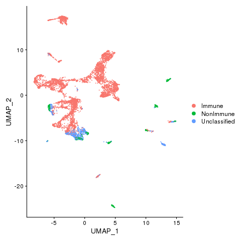
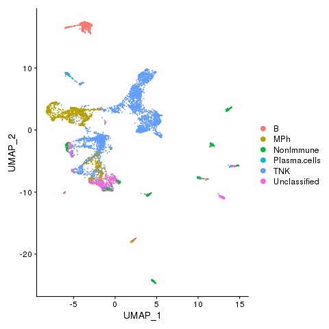
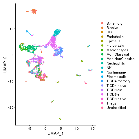
Now we can visualize the cell type classifications at many different levels:
kidney <- AddMetaData(kidney, metadata = celltypes$Immune, col.name = "immmune")
kidney <- SetIdent(kidney, value = "immmune")
png(filename = "fls/plot1_amp.png")
DimPlot(kidney)
dev.off()
Immune, Nonimmune (if any) and unclassified cells
kidney <- AddMetaData(kidney, metadata = celltypes$CellTypes, col.name = "celltypes")
kidney <- SetIdent(kidney, value = "celltypes")
png(filename = "fls/plot2_amp.png")
DimPlot(kidney)
dev.off()
Cell types
kidney <- AddMetaData(kidney, metadata = celltypes$CellStates, col.name = "cellstates")
kidney <- SetIdent(kidney, value = "cellstates")
png(filename = "fls/plot3_amp.png")
DimPlot(kidney)
dev.off()
Cell states
Identify immune marker genes (IMAGES)
# Downsample just the immune cells
kidney.small <- kidney[, !celltypes$CellStates %in% c("NonImmune", "Fibroblasts", "Unclassified",
    "Endothelial", "Epithelial")]

# Find protein markers for all clusters, and draw a heatmap
markers <- FindAllMarkers(kidney.small, only.pos = TRUE, verbose = F, logfc.threshold = 1)
require(dplyr)
top5 <- markers %>% group_by(cluster) %>% top_n(n = 5, wt = avg_logFC)
png(filename = "fls/plot4_amp.png", width = 640, height = 640)
DoHeatmap(kidney.small, features = unique(top5$gene), angle = 90)
dev.off()
Immune marker genes
Run MASC
Meta_mapped = M[match(colnames(kidney), M$cell_name), ]
Meta_mapped$CellStates = celltypes$CellStates
Meta_mapped$disease = factor(Meta_mapped$disease)
Q = MASC(dataset = Meta_mapped, cluster = Meta_mapped$CellStates, contrast = "disease", random_effects = c("plate",
    "lane", "sample"))
MASC results reveals that fibroblasts, plasma cells and B memory cells are enriched (p value < 0.05) for disease.
| cluster | size | model.pvalue | diseaseSLE.OR | diseaseSLE.OR.95pct.ci.lower | diseaseSLE.OR.95pct.ci.upper |
|---|---|---|---|---|---|
| B.memory | 391 | 0.0197539 | 3.041576e+00 | 1.1841285 | 7.812654e+00 |
| B.naive | 144 | 0.4652596 | 1.548526e+00 | 0.4932181 | 4.861810e+00 |
| DC | 160 | 0.0536208 | 2.346694e+00 | 1.0278135 | 5.357951e+00 |
| Endothelial | 30 | 0.2290332 | 1.183979e+01 | 0.1021348 | 1.372508e+03 |
| Epithelial | 89 | 0.5615659 | 6.424482e-01 | 0.1488724 | 2.772440e+00 |
| Fibroblasts | 360 | 0.0174935 | 3.926459e+00 | 2.5047560 | 6.155124e+00 |
| Macrophages | 356 | 0.1061625 | 4.700437e-01 | 0.1959415 | 1.127587e+00 |
| Mon.Classical | 247 | 0.6346884 | 8.482458e-01 | 0.4416789 | 1.629059e+00 |
| Mon.NonClassical | 658 | 0.7360915 | 8.693916e-01 | 0.3903675 | 1.936231e+00 |
| Neutrophils | 11 | 0.3806773 | 1.800080e-02 | 0.0000020 | 1.590775e+02 |
| NK | 562 | 0.2814722 | 6.046977e-01 | 0.2470403 | 1.480160e+00 |
| NonImmune | 112 | 0.1608263 | 7.817140e-02 | 0.0021302 | 2.868614e+00 |
| Plasma.cells | 93 | 0.0055213 | 5.387766e+06 | 0.0000000 | 1.579379e+25 |
| T.CD4.memory | 283 | 0.5351536 | 6.933100e-01 | 0.2284183 | 2.104379e+00 |
| T.CD4.naive | 459 | 0.4627315 | 7.488830e-01 | 0.3546322 | 1.581429e+00 |
| T.CD8.cm | 482 | 0.1776758 | 1.917053e+00 | 0.7686826 | 4.781025e+00 |
| T.CD8.em | 1196 | 0.7985566 | 1.107881e+00 | 0.5097435 | 2.407877e+00 |
| T.CD8.naive | 39 | 0.8117720 | 1.132623e+00 | 0.4022482 | 3.189161e+00 |
| T.regs | 84 | 0.6186262 | 1.571148e+00 | 0.2607223 | 9.467957e+00 |
| Unclassified | 717 | 0.8900750 | 9.198574e-01 | 0.2840429 | 2.978908e+00 |
Save results
saveRDS(kidney, file = "fls/amp_kidney_signac.rds")
saveRDS(Q, file = "fls/amp_kidney_MASC_result.rds")
saveRDS(celltypes, file = "fls/amp_kidney_celltypes.rds")
Session Info
## R version 4.0.0 (2020-04-24)
## Platform: x86_64-pc-linux-gnu (64-bit)
## Running under: CentOS Linux 7 (Core)
##
## Matrix products: default
## BLAS/LAPACK: /usr/lib64/libopenblasp-r0.3.3.so
##
## locale:
##  [1] LC_CTYPE=en_US.UTF-8       LC_NUMERIC=C
##  [3] LC_TIME=en_US.UTF-8        LC_COLLATE=en_US.UTF-8
##  [5] LC_MONETARY=en_US.UTF-8    LC_MESSAGES=en_US.UTF-8
##  [7] LC_PAPER=en_US.UTF-8       LC_NAME=C
##  [9] LC_ADDRESS=C               LC_TELEPHONE=C
## [11] LC_MEASUREMENT=en_US.UTF-8 LC_IDENTIFICATION=C
##
## attached base packages:
## [1] stats     graphics  grDevices utils     datasets  methods   base
##
## loaded via a namespace (and not attached):
##  [1] knitr_1.31        magrittr_2.0.1    R6_2.5.0          ragg_1.1.1
##  [5] rlang_0.4.10      fastmap_1.1.0     highr_0.8         stringr_1.4.0
##  [9] tools_4.0.0       xfun_0.21         jquerylib_0.1.3   htmltools_0.5.1.1
## [13] systemfonts_1.0.1 yaml_2.2.1        assertthat_0.2.1  digest_0.6.27
## [17] rprojroot_2.0.2   pkgdown_1.6.1     crayon_1.4.1      textshaping_0.3.1
## [21] formatR_1.7       sass_0.3.1        fs_1.5.0          memoise_2.0.0
## [25] cachem_1.0.3      evaluate_0.14     rmarkdown_2.7     stringi_1.5.3
## [29] compiler_4.0.0    bslib_0.2.4       desc_1.2.0        jsonlite_1.7.2