Cell type classification with SignacX: CITE-seq PBMCs from 10X Genomics
Compiled 2021-03-02
Source:vignettes/signac-Seurat_CITE-seq.Rmd
signac-Seurat_CITE-seq.RmdIn Figure 2-3 of the pre-print, we validated Signac with CITE-seq PBMCs. Here, we reproduced that analysis with Seurat, and provide interactive access to the data here. There are three parts to this vignette: Seurat, SignacX and then visualization. We use an example PBMCs CITE-seq data set from 10X Genomics.
Seurat
Start with the standard pre-processing steps for a Seurat object.
Download data from 10X Genomics.
dir.create("fls")
download.file("https://cf.10xgenomics.com/samples/cell-exp/3.0.0/pbmc_10k_protein_v3/pbmc_10k_protein_v3_filtered_feature_bc_matrix.h5",
    destfile = "fls/pbmc_10k_protein_v3_filtered_feature_bc_matrix.h5")
Create a Seurat object, and then perform SCTransform normalization. Note:
- You can use the legacy functions here (i.e., NormalizeData, ScaleData, etc.), use SCTransform or any other normalization method (including no normalization). We did not notice a significant difference in cell type annotations with different normalization methods.
- We think that it is best practice to use SCTransform, but it is not a necessary step. SignacX will work fine without it.
# load dataset
E = Read10X_h5(filename = "fls/pbmc_10k_protein_v3_filtered_feature_bc_matrix.h5")
pbmc <- CreateSeuratObject(counts = E$`Gene Expression`, project = "pbmc")

# run sctransform
pbmc <- SCTransform(pbmc)
Perform dimensionality reduction by PCA and UMAP embedding. Note:
- SignacX actually needs these functions since it uses the nearest neighbor graph generated by Seurat.
# These are now standard steps in the Seurat workflow for visualization and clustering
pbmc <- RunPCA(pbmc, verbose = FALSE)
pbmc <- RunUMAP(pbmc, dims = 1:30, verbose = FALSE)
pbmc <- FindNeighbors(pbmc, dims = 1:30, verbose = FALSE)
SignacX
Load the package
Generate SignacX labels for the Seurat object. Note:
- Optionally, you can do parallel computing by setting num.cores > 1 in the Signac function.
- Run time is ~10-20 minutes for <100,000 cells.
# Run Signac
labels <- Signac(pbmc, num.cores = 4)
celltypes = GenerateLabels(labels, E = pbmc)
Can we make Signac faster?
Sometimes, training the neural networks takes a lot of time. To make Signac faster, we implemented SignacFast which uses an ensemble of pre-trained neural network models. Note:
- SignacFast uses an ensemble of 1,800 pre-calculated neural networks using the GenerateModels function together with the training_HPCA reference data.
- Features that are absent from the single cell data and present in the neural network are set to zero.
# Run Signac
labels_fast <- SignacFast(pbmc)
celltypes_fast = GenerateLabels(labels_fast, E = pbmc)How does SignacFast compare to Signac?
| B | MPh | TNK | Unclassified | |
|---|---|---|---|---|
| B | 550 | 0 | 0 | 0 |
| MPh | 0 | 2178 | 0 | 0 |
| TNK | 0 | 0 | 4914 | 0 |
| Unclassified | 0 | 4 | 2 | 217 |
Visualizations
Now we can visualize the cell type classifications at many different levels: Immune and nonimmune
pbmc <- AddMetaData(pbmc, metadata = celltypes_fast$Immune, col.name = "immmune")
pbmc <- SetIdent(pbmc, value = "immmune")
png(filename = "fls/plot1_citeseq.png")
DimPlot(pbmc)
dev.off()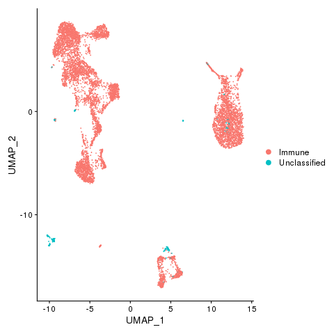
Immune, Nonimmune (if any) and unclassified cells
pbmc <- AddMetaData(pbmc, metadata = celltypes$L2, col.name = "celltypes")
pbmc <- SetIdent(pbmc, value = "celltypes")
png(filename = "fls/plot2_citeseq.png")
DimPlot(pbmc)
dev.off()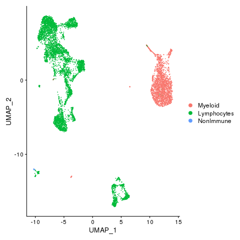
Myeloid and lymphocytes
pbmc <- AddMetaData(pbmc, metadata = celltypes$CellTypes, col.name = "celltypes")
pbmc <- SetIdent(pbmc, value = "celltypes")
png(filename = "./fls/plot3_citeseq.png")
DimPlot(pbmc)
dev.off()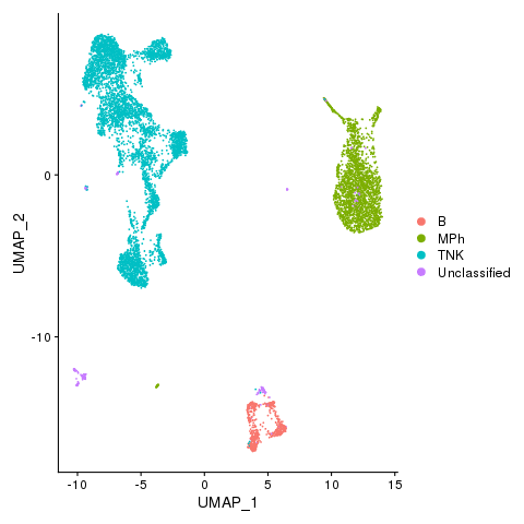
Cell types
pbmc <- AddMetaData(pbmc, metadata = celltypes$CellTypes_novel, col.name = "celltypes_novel")
pbmc <- SetIdent(pbmc, value = "celltypes_novel")
png(filename = "./fls/plot4_citeseq.png")
DimPlot(pbmc)
dev.off()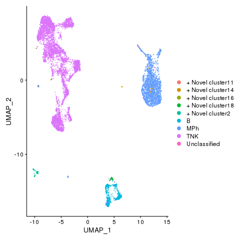
Cell types with novel populations
pbmc <- AddMetaData(pbmc, metadata = celltypes$CellStates, col.name = "cellstates")
pbmc <- SetIdent(pbmc, value = "cellstates")
png(filename = "./fls/plot5_citeseq.png")
DimPlot(pbmc)
dev.off()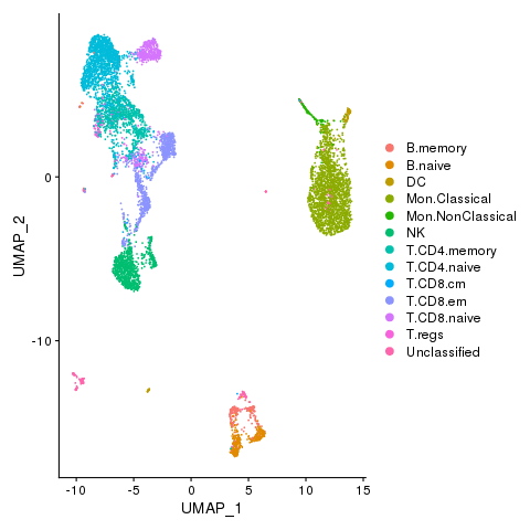
Cell states
Identify differentially expressed genes between cell types.
pbmc <- SetIdent(pbmc, value = "celltypes")

# Find markers for all clusters, and draw a heatmap
markers <- FindAllMarkers(pbmc, only.pos = TRUE, verbose = F, logfc.threshold = 1)
library(dplyr)
top5 <- markers %>% group_by(cluster) %>% top_n(n = 5, wt = avg_logFC)

png(filename = "./fls/plot9_citeseq.png", width = 640, height = 720)
DoHeatmap(pbmc, features = unique(top5$gene), angle = 90)
dev.off()
Immune marker genes - cell types
pbmc <- SetIdent(pbmc, value = "cellstates")
# Find markers for all clusters, and draw a heatmap
markers <- FindAllMarkers(pbmc, only.pos = TRUE, verbose = F, logfc.threshold = 1)
top5 <- markers %>% group_by(cluster) %>% top_n(n = 5, wt = avg_logFC)
png(filename = "./fls/plot6_citeseq.png", width = 640, height = 720)
DoHeatmap(pbmc, features = unique(top5$gene), angle = 90)
dev.off()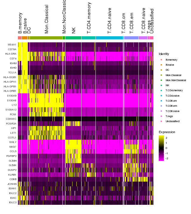 Add protein expression information
pbmc[["ADT"]] <- CreateAssayObject(counts = E$`Antibody Capture`[, colnames(E$`Antibody Capture`) %in%
    colnames(pbmc)])
pbmc <- NormalizeData(pbmc, assay = "ADT", normalization.method = "CLR")
pbmc <- ScaleData(pbmc, assay = "ADT")
Identify differentially expressed proteins between clusters
DefaultAssay(pbmc) <- "ADT"
# Find protein markers for all clusters, and draw a heatmap
adt.markers <- FindAllMarkers(pbmc, assay = "ADT", only.pos = TRUE, verbose = F)
png(filename = "./fls/plot7_citeseq.png", width = 640, height = 720)
DoHeatmap(pbmc, features = unique(adt.markers$gene), angle = 90)
dev.off()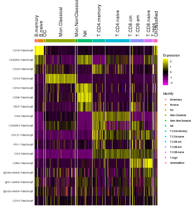
Immune marker genes
Save results
saveRDS(pbmc, file = "fls/pbmcs_signac_citeseq.rds")
saveRDS(celltypes, file = "fls/celltypes_citeseq.rds")
saveRDS(celltypes_fast, file = "fls/celltypes_fast_citeseq.rds")
Session Info
## R version 4.0.0 (2020-04-24)
## Platform: x86_64-pc-linux-gnu (64-bit)
## Running under: CentOS Linux 7 (Core)
##
## Matrix products: default
## BLAS/LAPACK: /usr/lib64/libopenblasp-r0.3.3.so
##
## locale:
##  [1] LC_CTYPE=en_US.UTF-8       LC_NUMERIC=C
##  [3] LC_TIME=en_US.UTF-8        LC_COLLATE=en_US.UTF-8
##  [5] LC_MONETARY=en_US.UTF-8    LC_MESSAGES=en_US.UTF-8
##  [7] LC_PAPER=en_US.UTF-8       LC_NAME=C
##  [9] LC_ADDRESS=C               LC_TELEPHONE=C
## [11] LC_MEASUREMENT=en_US.UTF-8 LC_IDENTIFICATION=C
##
## attached base packages:
## [1] stats     graphics  grDevices utils     datasets  methods   base
##
## loaded via a namespace (and not attached):
##  [1] knitr_1.31        magrittr_2.0.1    R6_2.5.0          ragg_1.1.1
##  [5] rlang_0.4.10      fastmap_1.1.0     highr_0.8         stringr_1.4.0
##  [9] tools_4.0.0       xfun_0.21         jquerylib_0.1.3   htmltools_0.5.1.1
## [13] systemfonts_1.0.1 yaml_2.2.1        assertthat_0.2.1  digest_0.6.27
## [17] rprojroot_2.0.2   pkgdown_1.6.1     crayon_1.4.1      textshaping_0.3.1
## [21] formatR_1.7       sass_0.3.1        fs_1.5.0          memoise_2.0.0
## [25] cachem_1.0.3      evaluate_0.14     rmarkdown_2.7     stringi_1.5.3
## [29] compiler_4.0.0    bslib_0.2.4       desc_1.2.0        jsonlite_1.7.2